The temporal evolution of dynamical systems, describing how they change over time, is fundamental for understanding a wide range of phenomena. However, accurately predicting their behaviour, especially over long durations, can be incredibly difficult. This complexity often stems from non-linear interactions, sensitivity to starting conditions, and the sheer volume of data these systems can generate. We will explore these challenges and potential solutions through an illustrative example.
| \( f \) | This is the symbol for a function. It is commonly used in algebra, and (multivariate) calculus. |
| \( ' \) | This is the symbol for the derivative of a function. If \(f(x)\) is a function, then \(f'(x)\) is the derivative of that function. |
| \( z \) | This symbol is for a function that represents a generic ordinary differential equation, meaning an equation that contains one or more ordinary derivatives. |
Consider some abstract ODE \( \htmlClass{sdt-0000000010}{z} \). To calculate its evolution over time (\( \htmlClass{sdt-0000000118}{t} \)), we need to differentiate \( \htmlClass{sdt-0000000010}{z} \) with respect to \( \htmlClass{sdt-0000000118}{t} \). We can express this differentiation using an arbitrary function for simplicity. Thus, we obtain a general equation:
\[\htmlClass{sdt-0000000010}{z} \htmlClass{sdt-0000000025}{'} = \htmlClass{sdt-0000000096}{f}(\htmlClass{sdt-0000000010}{z})\]
Note that \(\htmlClass{sdt-0000000010}{z} \htmlClass{sdt-0000000025}{'}\) in this case means a derivative with respect to time. It is often abbreviated as \(\overset{.}{\htmlClass{sdt-0000000010}{z}}\)
Consider a more concrete example using an ODE with two components \(x\) and \(y\). We can obtain these components' evolution by again differentiating with time. Using the general equation for discussed above, we obtain:
\[ \htmlClass{sdt-0000000096}{f}(\htmlClass{sdt-0000000010}{z}) = \htmlClass{sdt-0000000096}{f}((\htmlClass{sdt-0000000003}{x}, \htmlClass{sdt-0000000017}{y})\htmlClass{sdt-0000000025}{'}) = ( \begin{array}{c} \htmlClass{sdt-0000000085}{g}(\htmlClass{sdt-0000000003}{x},\htmlClass{sdt-0000000017}{y}) \\ \htmlClass{sdt-0000000020}{z}(\htmlClass{sdt-0000000003}{x},\htmlClass{sdt-0000000017}{y}) \end{array} )\]
where \(\htmlClass{sdt-0000000085}{g}\) and \(\htmlClass{sdt-0000000020}{z}\) are functions for computing the derivatives of the components. One might notice that these components are coupled as we cannot modify one without changing the other. More precisely, the derivative for each component is as follows:
\[\begin{align*} \overset{.}{x} &= \htmlClass{sdt-0000000085}{g}(\htmlClass{sdt-0000000003}{x},\htmlClass{sdt-0000000017}{y}) = -\htmlClass{sdt-0000000003}{x}(\htmlClass{sdt-0000000003}{x}^2 + \htmlClass{sdt-0000000017}{y}^2)^3 + \htmlClass{sdt-0000000003}{x} - \htmlClass{sdt-0000000017}{y} \\ \overset{.}{y} &= \htmlClass{sdt-0000000020}{z}(\htmlClass{sdt-0000000003}{x},\htmlClass{sdt-0000000017}{y}) = -\htmlClass{sdt-0000000017}{y}(\htmlClass{sdt-0000000003}{x}^2 + \htmlClass{sdt-0000000017}{y}^2)^3 + \htmlClass{sdt-0000000017}{y} + \htmlClass{sdt-0000000003}{x} \end{align*}\]
These equations might seem fairly complex but can be simplified using polar coordinates by expressing the components using the radius \(\htmlClass{sdt-0000000063}{r}\) and angle \(\htmlClass{sdt-0000000024}{\theta}\) at each time step. After simplification, we obtain the derivatives as:
\[\begin{align*} \overset{.}{\htmlClass{sdt-0000000063}{r}} &= -\htmlClass{sdt-0000000063}{r}^{3} + \htmlClass{sdt-0000000063}{r} \\ \overset{.}{\htmlClass{sdt-0000000024}{\theta}} &= 1 \end{align*}\]
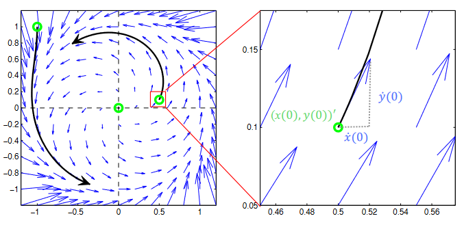
A benefit of this notation is that the two components are decoupled. This allows us to interpret the system easily. Regardless of the notation, the graph on the left is obtained due to the ODE's evolution. The graph on the right is a zoomed-in view of the same.